The macroeconomic model for Aggregate Demand and Aggregate Supply differs from the microeconomic model in the fact that the AD/AS model represents all goods and not just one single good. It takes into account the price level of all goods as well as the overall aggregate output of the economy.
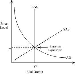
Aggregate Demand (AD) represents the demand side of the economy. Long-run Aggregate Supply (LAS) represents the most output that an economy can sustain. Short-run Aggregate Supply (SAS) represents the supply of the economy in the short run. These three components can be explained separately and brought together to represent some equilibrium price level and aggregate output.
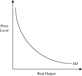
Aggregate Demand is the relationship between the aggregate price level and the quantity of output. AD is similar to the law of demand that already exists but the factors that affect AD are slightly different than demand. The factors that affect AD are household consumption, government spending, investment, and net exports. It is important to note that AD is the same in both the short run and the long run. Aggregate Demand represents how a change in a certain price level will change expenditures on all services and goods in an economy. There are several components that make up AD and explain how it works. These are:
- The Effects of Price on Aggregate Demand
- Other Factors Besides Price Effecting Aggregate Demand
- The Multiplier Effect
The AD curve is downward sloping due to the interest rate effect, the international effect, and the wealth effect.
The Effects of Aggregate Demand
Aggregate expenditures and price are inversely related. A rise in price level will cause a decrease in aggregate expenditures and a decrease in price level will cause an increase in aggregate expenditures. There are three things that explain why falling price levels increase aggregate expenditures.
They are:
- The Wealth Effect: This says that a rise in the price level will make people who have money and other financial assets feel poorer. They then buy less, and the opposite is true if the price level were to fall- people would buy more. If people feel poorer and since consumption is a part of AD, then aggregate expenditures will decrease, thus decreasing the quantity demanded.
- The International Effect: This states that as the price of our goods go up -and become more expensive to foreigners- net exports will fall. In addition, imports will increase because foreign goods will seem cheaper than the goods at home whose prices have risen. Since net exports will fall and this is a part of AD, then overall aggregate expenditures will decrease.
- The Interest Rate Effect: This says that as price increases, interest rates will increase causing investments to decrease. If prices are higher, then people will have less money because they will be forced to spend more. If interest rates are higher, people will be less willing to put what little money they have into investments. Since Investments are part of the aggregate demand, the quantity of aggregate expenditures will go down, showing a negative relationship between price and aggregate expenditures.
Shift Factors of Aggregate Demand
Aggregate Demand can increase or decrease depending on several things. In effect, these things will cause shifts up or down in the AD curve. These include:
- Exchange Rates: When a country's exchange rate increases, then net exports will decrease and aggregate expenditure will go down at all prices. This means that AD will decrease.
- Distribution of Income: This is directly related to wages and profits. When worker's real wages increase, then people will have more money on their hands because their overall income has increased. When this happens they tend to consume more causing the consumption expenditures to increase.
- Expectations: Consumers tend to have certain expectations about the future of the economy and will adjust their spending accordingly. If they would expect the economy to not do so well in the future, saving would increase thus decrease overall expenditures. Rising price levels will cause aggregate demand to increase. If consumers foresee the price level to rise in the near future, they might just go out and buy that good now, increasing the consumption expenditures in AD. Many different expectations have the capacity to increase or decrease aggregate demand and it is not always clear as to how this will happen.
- Foreign Income: This relates U.S. economic output with the income of its trading partners in the world. When foreign income rises, U.S. exports will increase causing aggregate demand to increase.
- Monetary and Fiscal Policies: The government has some ability to impact AD. They can spend money or increase taxes in order to influence how consumers spend or save. An expansionary fiscal policy causes AD to increase, while a contractionary monetary policy causes AD to decrease.
The Multiplier Effect
In microeconomics, things are assumed to be constant; However, in macroeconomics, the after effects are also taken into account. The Multiplier Effect discusses the repercussions of initial changes in expenditures which amplify the initial effects. A change in price level has the potential to affect many different parts of the economy either in positive or in adverse ways depending on how the effects happen. The multiplier effect takes the initial wealth, international, and interest rate effects and amplifies these original effects. For example, a Mercedes plant locating in a city may create jobs, revenue, and knowledge spillovers. This can help to improve the local economy through the multiplier effect.
Long-Run Aggregate Supply
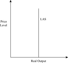
The Long-Run Aggregate Supply (LAS) represents the relationship between the price level and output in the long-run. It differs from the Short-Run Aggregate Supply (SAS) in that no input prices are assumed to be constant. Thus, LAS is a representation of potential output.
Since the LAS is potential output it is shifted by the factors which affect potential output, such as:available resources, capital, entrepreneurship, and technological developments. Where LAS is affects whether policies are focused on short-run or long-run issues.
The LAS curve is vertical because it shows potential output and when this happens all prices, even input prices, rise when a rise in price level occurs.
Short-Run Aggregate Supply
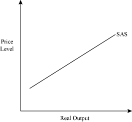
Short-run Aggregate Supply (SAS) shows the different quantities of real output in the short-run that will be supplied at different prices. There are several things that affect the SAS curve.
- The Effects of Price on the Short-Run Aggregate Supply Curve: As price increases, the quantity supplied will also increase, indicating a postive relationship between price and quantity supplied.
- Other Things Besides Price that Effect Short-Run Aggregate Supply
The SAS curve is upward sloping because firms tend to increase price levels when demand increases and because in auction markets there are upward sloping supply curves. There are two main theories to explain why the SAS curve is upward sloping and they are the sticky-wage model and the sticky-price model.
Other Things Besides Price that Effects Short-Run Aggregate Supply
- Aggregate Price: This says that as price increases, the quantity supplied will also increase, indicating a positive relationship.
- Input Costs: If input costs such as wages increase, then SAS will decrease because the producers will decrease supply.
- Technology: As technology continues to improve, SAS will increase.
- Government Policy on Taxes: If business or corporate taxes are lowered, then SAS will increase.
- Investments: If investments were to increase, SAS will increase. On the other hand, if investments were to fall, then SAS will decrease.
What all of these factors have in common is that any increase in input prices will decrease SAS and any decreases in input prices will increase production in the SAS. So, anything that is able to change the factor costs will be a shift factor of Short-Run Aggregate Supply.
Equilibrium
Aggregate Demand (AD), Short-run Aggregate Supply (SAS), and Long-run Aggregate Supply (LAS) can all be represented on a graph as a curve. The AD curve is downward sloping, the SAS curve is upward sloping, and the LAS is a vertical line. The point at which either AD intersects SAS or AD intersects LAS is called the equilibrium point.
- Short-Run Equilibrium
- Long-Run Equilibrium
Recessionary Gap:
Sometimes AD is below the potential output because not all of the resources in the economy are being fully used. The amount that equilibrium output is below potential output is called the recessionary gap. For example if potential output is 1,500,000 and the equilibrium output is 1,000,000, then the recessionary gap is 500,000.
Inflationary Gap:
This occurs when the income is greater than the potential output. There is more demand than is able to be produced. During these times, inflation rises and trade worsens. To help control inflationary gaps, the government will use fiscal or monetary policies.
Beyond Potential:
The situation of the inflationary gap cannot last long because resources are being over utilized and will eventually return to potential output.
Short-Run Equilibrium
The equilibrium in the short-run is shown by the intersection of the Aggregate Demand (AD) curve and the Short-Run Aggregate Supply (SAS) curve. When either AD or SAS shifts, the equilibrium point is changed. For example, in Graph 1, a shift to the right of the AD curve will cause the equilibrium output as well as the price level to increase. And if the AD curve were to shift to the left, as in Graph 2, the opposite would be true: output and price level will decrease.
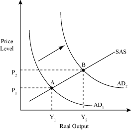
Graph 1
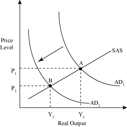
Graph 2
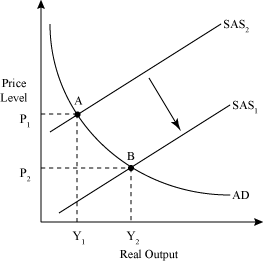
A shift to the left in SAS, as shown in Graph 3, will cause the price level to rise while equilibrium output will decrease. And a shift to the right, as shown in Graph 4, will decrease price level and increase output.
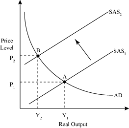
Graph 3
Long-Run Equilibrium
The equilibrium in the long-run is shown by the intersection of the AD curve, the SAS curve, and the Long-Run Aggregate Supply (LAS) curve. Since LAS represents potential output, a shift in the AD curve will only result in a change in price level: a shift to the right increasing price level and a shift to the left decreasing price level. If an economy is said to be in long-run equilibrium, then Real GDP is at its potential output, the actual unemployment rate will equal the natural rate of unemployment (about 6%), and the actual price level will equal the anticipated price level.